An in-depth guide on the basics of Oscilloscopes
An oscilloscope is a very handy item in the electrical and electronic engineers toolbox. An oscilloscope is used to measure and visualize electrical signals. In its most common application, an oscilloscope measures the electrical potential difference, or voltage, at a given point to which the probe is connected. An oscilloscope is also capable of measuring non-electrical signals, such as sound intensity, by converting a signal into electrical form.
As an initial example, here is a visualization of the signal produced by a 9V battery. The horizontal dotted line represents 9V and the blue line represents the voltage produced by the battery. As we can see, this battery produces slightly more than 9V.
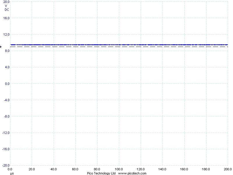
Figure 1 – 9V Battery – 20 V @ 20 us/div
The oscilloscope visualization can be adjusted by changing the scale on either axis. The horizontal axis represents the period of time over which the measurements are taken. The vertical axis represents the measured voltage. The vertical axis can also be shifted positively or negatively to potentially provide a more meaningful visualization to the engineer.
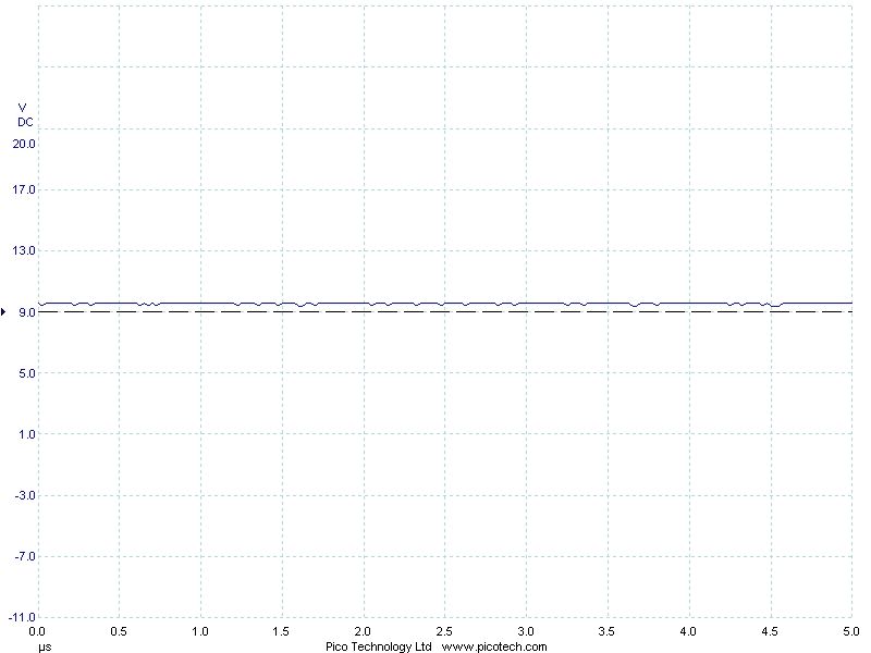
Figure 2 – 9V Battery – 20 V @ 500 ns/div, shifted negatively
An important aspect of acquiring an accurate signal is ensuring that the oscilloscope is adequately connected to a ground. Not only can this provide safety when in contact with electrical signals but also it will allow interference to be distributed away from the signal that we are interested in measuring. Here are two visualizations of the same signal; the first signal is not grounded while the second is grounded and is somewhat clearer.
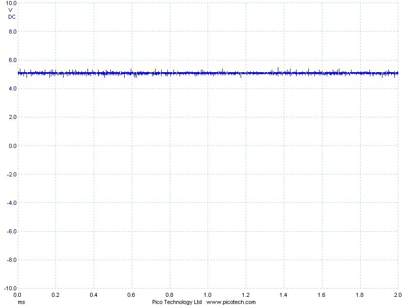
Figure 3 – Electrical signal without connection to ground
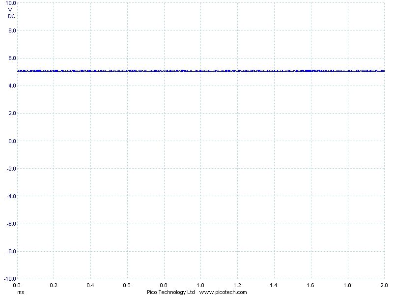
Figure 4 – Electrical signal with connection to ground
There is even a measurable amount of electrical signals in the air or free space around us. These signals are more commonly known as electromagnetic fields. In this case, the oscilloscope reads between +/- 7 mV when the probe is held in free space.
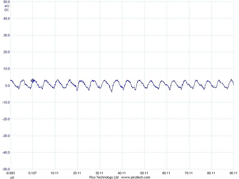
Figure 5 – EMF in Free Space – 50 mV @ 10 us/div
Electromagnetic fields are produced by electrical devices and can be significantly greater near sources of electrical signals such as power supplies. For this example, the oscilloscope probe is positioned approximately two centimeters away from a 12V/DC power supply. Now, we can see the voltage being measured by the oscilloscope is +/- 200 mV.
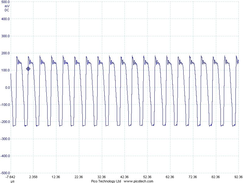
Figure 6 – EMF near power supply – 500 mV @ 10 us
In relation to digital electronic devices, an oscilloscope can be an invaluable tool in the testing of signals that are produced by a given device. In doing this testing, an engineer can determine whether or not a device is producing the appropriate or expected signal. Here is an example of a digital device producing a repeating signal which raises the voltage to 5V for a period and then 0V for a period.
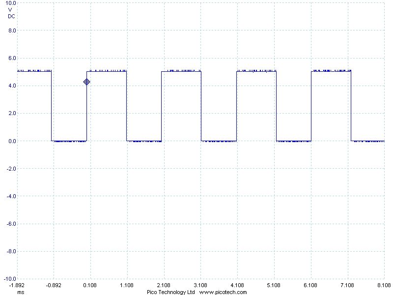
Figure 7 – Digital signal – 10 V @ 1 ms/div
In a practical application, a digital signal will represent a series of one's and zero's to form binary data. This type of signal comprises the most basic representation of data communication between digital devices, which are intrinsic to everyday life. While the signal in the next example shows just 8 bits over 1 ms, a more common rate of producing this type of binary signal is 100 bits per millisecond.
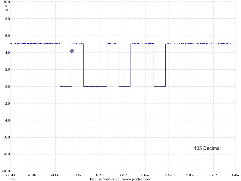
Figure 8 – Digital signal – Binary representation of Decimal 105
Comments (1) One Response to "Oscilloscope Basics"
- Oscilloscope Rental says:September 28, 2009 at 5:51 am
Oscilloscope power supply lifespan is very important. Shortage of power source may affect its component not to function properly and might give wrong reading.
Reply